A Comparison of Airfoils for Pylon Racing Models |
During the 1980s, airfoils with reflexed camber lines (like the E 22x and the MH 1x series) appeared in pylon racing models and were soon dominating the scene in Germany. In recent years, a new and quite different airfoil shape could be seen regularly on pylon racing contests: all these new airfoils had the location of the maximum thickness further downstream, resulting in a rapid closure of the airfoil shape at the trailing edge. The aerodynamic design of these airfoils was targeted at extremely large areas of laminar flow in order to minimize the friction drag. The designers were well aware of the fact, that there would be a penalty in terms of drag at lower Reynolds numbers and that advanced manufacturing techniques would be needed to realize the theoretically possible performance improvements.
One of the first airfoils for model aircraft application of this type was the DU 86-084/18, developed at the University of Delft in the Netherlands, and used in sailplane models of the F3B class. After a first wave of rumors and success stories, this airfoil is rarely seen today. When the recommended turbulators (transition strips) were used, the low drag figures of this airfoil could be realized, but it was no real improvement, when compared with the more conventional designs. In the meantime, more DU airfoils have been developed and were used in pylon racing models - the DU 91090 is one of this family. Unfortunately the author has no published source for the airfoil coordinates available.
In 1992, I developed a whole family of extreme laminar flow airfoil sections, which were intended to be incorporated into the F3D models of the German pylon racing teams for the upcoming world championships. When the championships were over, the coordinates of these sections were published in [6]. Today, it is mainly the MH 24 which is used on numerous racing models, not only because it fits the FAI regulations concerning wing thickness quite well. Although most models were built in moulds, using composite materials, these airfoils can also be used on foam sandwich wings, when a good surface finish is applied and when the shape is checked carefully with templates.
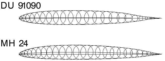
Geometry of the two airfoils DU 91090 and MH 24
Both airfoils are approximately 9% thick, but the MH 24 has much more camber. The locations of maximum thickness and maximum camber of the Delft airfoil are further back than the values of the MH airfoil.
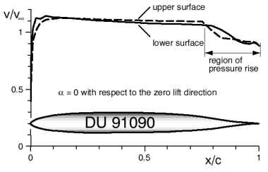 |
The velocity distribution of the DU 91090 shows the laminar flow region with a nearly constant velocity, followed by a steep pressure rise, which can cause laminar flow separation and drag increase at small Reynolds numbers. |
As it was quickly learned, it is not sufficient to compare the pure airfoil polars and, as a consequence, a complete simulation environment was composed to make a realistic comparison possible.
During the operation of F3D pylon racing models, the airfoils DU 91090 and MH 24 are used in a narrow band of operating conditions only. The wing of a typical contest model flies at Reynolds numbers between 600'000 and 1'500'000. When the model is cruising with a flight speed of 80 m/s, the lift coefficient is between zero and 0.05, during the turns a maximum lift coefficient of 0.6 is rarely exceeded. Flaps could be useful, but they are very difficult to adjust and the gain in performance is small. At first glance, the true operating conditions are not so clearly obvious or well defined.
The analysis of the airfoils was mainly performed with Mark Drela's XFOIL, Version 5.4, because it seems to be better suited to predict separation and laminar separation bubbles. The results were also checked against Eppler's airfoil analysis program, which predicts the width and location of the laminar bucket better. Wind tunnel results were not available.
The downstream location of the maximum thickness of these airfoils results in extended laminar flow regions, but also in a rapid closure of the airfoil shape at the trailing edge. The velocity distribution of the DU 91090 shows the steep pressure rise in the rear part of the airfoil, which can only be overcome without separation, when the flow is turbulent. Thus, both airfoils need a turbulator to force the transition before the flow reaches the closure region of the airfoil. The location of the transition strip should be optimized for each airfoil: if it is located too far forward, the transition takes place early and the friction drag is higher than necessary. When it is to far downstream, it cannot force transition efficiently or must be very thick, which can result increased drag. Additionally, there is a Reynolds number effect: when the Reynolds number is increased, the natural transition tends start earlier and, at some high enough Reynolds number, the turbulator is not necessary anymore. For the MH 24, natural transition begins to onset at Reynolds numbers above 1'200'000. In order to find the optimum location of the turbulator for each airfoil, systematic, numerical studies were performed. For different Reynolds numbers, the transition was fixed at different chordwise locations, advancing in 1% chord steps. Typical results for the MH 24 under zero lift conditions are shown below. The plot shows the drag coefficient Cd for different, constant Reynolds numbers, plotted versus transition (turbulator) location. The typical curve shows high drag values when the turbulator is to far forward, which decreases nearly linearly when the transition is shifted towards the rear. When the position of the turbulator reaches the point of laminar separation, the curve flattens and the drag coefficient begins to rise again: the transition strip in getting immersed in the region of separated flow. Finally, when the strip is moved completely into the dead water wake, it cannot influence the drag coefficient anymore and, Cd stays constant.
Drag coefficient of the MH 24, depending on transition location. The flat plate
coefficients are valid for a Reynolds number of 1'000'000.
It is quite convenient, that the minimum drag of this airfoil occurs at the same transition location, nearly independent of the Reynolds number. Therefore it is possible to select a single, optimum location for the transition strip; in case of the MH 24, this is approximately at 85% of the chord.
Using this method, the optimum transition locations were selected for both airfoils. In order to make sure, that transition really occurs, the transition was finally moved forward by 1% of the chord.
| DU 91090 | MH 24 | |
|---|---|---|
| transition on upper surface | 75% x/c | 84% x/c |
| transition on lower surface | 81% x/c | 86% x/c |
If a minimum Reynolds number of 1'000'000 is always maintained, a transition strip can eventually be omitted.
Using XFOIL, airfoil polars were calculated for different Reynolds numbers. From the plots below it can be seen, that the Delft airfoil, with its low amount of camber, works similar to a symmetrical section. The polar reaches down to negative lift coefficients and the moment coefficient is nearly zero, which makes it possible to use very small horizontal tails.
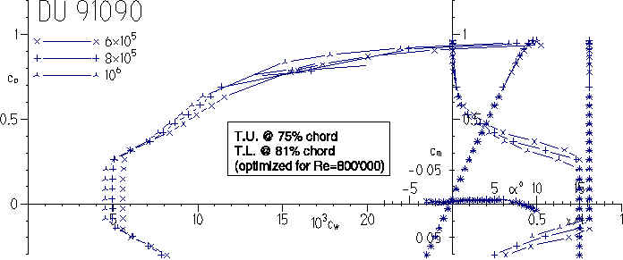
Airfoil polar of the DU 91090 with optimum transition.
The polars of the MH 24 are shifted towards higher lift coefficients and show low drag values between Cl=0 and Cl=0.6. The higher moment coefficient would require larger stabs, but in reality even the smaller horizontal tails are large enough, because they are usually designed for safe operation during take off and landing conditions. The maximum lift coefficient of both airfoils is nearly identical. The lower drag coefficient of the MH 24 is surely related to the transition location, which could not be moved further backwards on the DU 91090 without increasing the drag due to separation.
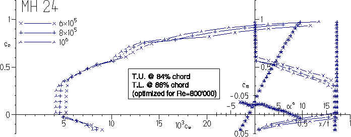
Airfoil polar of the MH 24 with optimum transition.
The drag of the airfoil is only one part of the total drag, which is increased by induced (wing planform) and parasitic drag (fuselage, tail, landing gear, engine cooling, linkages, ...). During the turns, the induced drag increases dramatically, whereas it is of no importance for a fast pylon racing model in level flight. A pylon race is a combination of level flight and turns, and the drag in the turns depends on the turn radius. With a fast model, it could be permissible to fly large turns and, on the other hand, it would be possible to use a high lift airfoil to fly very tight turns with high induced drag, but of short duration. Thus, it was necessary to perform a simulation of all these possibilities in order to make a fair comparison of the airfoils. As the model size is quite well defined by the FAI rules, no attempt was made to optimize the model itself for each airfoil (it is felt, that these resulting differences will be of minor importance).
For a realistic comparison, it was decided to write a small computer program, which should provide a simulation of a complete pylon race. The model should «fly» around the prescribed course, following these steps:
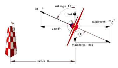 |
Forces acting on the model during the turns. For a stationary turn (no climbing or diving), the inward component of the lift must balance the radial force, and the vertical component must be equal to the mass force. |
The two airfoils of interest have different moment coefficients. Thus it is possible to use a smaller horizontal tail with the DU 91090 airfoil, which means less drag. In order to provide a fair comparison, the size of the tailplane was adapted to the airfoils moment coefficient, but the final results show, that there are only very small effects in terms of overall performance. One of the reasons is, that the FAI rules prescribe a wing section on 0.34 m², which increases the surface of the wing accordingly, when the size of the tailplane is reduced. The simulation program uses a simple scheme, depicted below, to determine the size of the tailplane. The scheme takes into account, that the tailplane must be able to control the plane during take off and landing as well as during high speed flight. For the DU 91090, the resulting tailplane has a size of only 0.021 m², whereas the model with the MH 24 requires a tailplane with an area of 0.055 m² (the distance between tailplane and the center of gravity has been held constant.
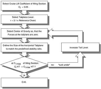 |
Approximate sizing procedure for the horizontal tailplane. |
To account for the 1/4 roll into and out of the turns, a rolling time of 0.25 seconds with an increase in airfoil drag of 10% was assumed. Also the induced drag was increased by 20% during this time. A comparison of results with, and without this additional drag shows, that the difference in total racing time is approximately 0.2 seconds only.
The internal combustion engine of an F3D model swallows approximately 5 liters of fuel per hour and the fuel weighs around 800 kg/m³. A topped up fuel tank of 0.2 liters feeds the engine for approximately 140 seconds (this means 1.7 liter per 100 km at 400 kW per liter displacement). The mass of the model is reduced by 0.08 kg during a race, which is not visible in the final results.
The simple aerodynamic model used in the simulation program contains a linear interpolation of the airfoil characteristics, depending on the Reynolds number. As the polars contain a dense distribution of points, the interpolation error is quite small. The induced drag coefficient Cdi of the wing is approximated by the simple formula
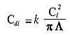 (1)
(1)
assuming a good wing design with k=1.1. For each time step the corresponding lift of the tailplane is calculated and induced drag is calculated using the same formula as for the wing. The friction drag of the tailplanes is included in the fuselage and interference drag. For a model with retractable landing gear the drag coefficient of the fuselage and tailplane was assumed to be 0.008 and for a fixed undercarriage (Quickie 500) a value of 0.011 was used (with respect to wing area). For the following simulations, all airfoil polars were calculated with XFoil 5.4 and optimized transition location, as described above.
Most of the simulations were conducted for standard conditions (at sea level), but also some test were made for different conditions. The density and viscosity of the air are calculated from ambient pressure and temperature and the performance of the engine is directly multiplied by the ratio of the current density divided by the sea level density.
The dependency between thrust and flight speed was either expressed by a simple, analytical function, or by interpolating data from a table of speed/rpm/thrust values. The thrust approximation was based on the formula
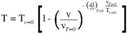 (2)
(2)
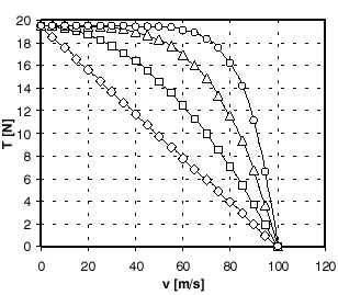
which needs the static thrust Tv=0, the flight speed where the thrust goes to zero vT=0 and the gradient dT/dV at this flight speed as input. The graph below shows some possible thrust curves coming from this formula.
|
|
A set of thrust curves calculated from formula (2) shows the possible curve shapes. The curves with squares and triangles are quite realistic. |
The second, interpolating approach made it possible to use experimental results for the simulation when they became available later, together with reliable engine data [more info].
In order to find the optimum lift coefficient for the turns, repeated runs of the program were conducted for the two airfoils and the corresponding models. The figure below shows some typical results of such runs. The current version of the program performs the search for the optimum lift coefficient automatically.
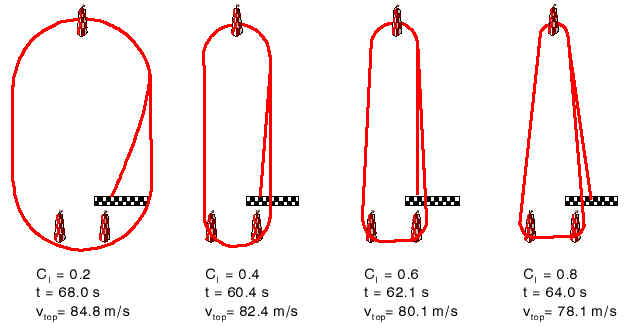
Some typical flight paths with different lift coefficients during
the turns and the resulting maximum speeds as well as the final racing times.
| By plotting the results versus the turn radius, we obtain another graph, shown on the right. The calculations were made for the MH 24 model and two turning strategies were compared: the optimal case, where the distance to the pylons is always 5 meters, and a more realistic case, where this 5 m distance is only maintained at the twin pylons. At the first pylon, the turn is beginning, when the model has reached the pylon, i.e. when the caller has signaled that the model has flown far enough to avoid a cut. It is clearly visible, that the best results are not obtained by flying extremely tight turns, but by turning at larger radii instead. |
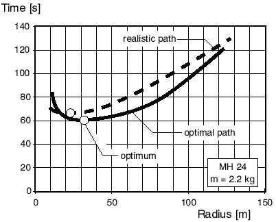 Racing times versus turn radius. |
| The table lists the main data of these models and the
possible race times.
It is interesting to note, that the MH 24 model races 3 seconds faster than its DU 91090 colleague - despite its disadvantage of having a horizontal tail of nearly twice the size of its rival. |
|
| If we look at the next graph, we can see, where the drag
comes from: we see, that there is no big difference in total drag
during the turns. The bar for the MH 24 model shows some drag of the
horizontal tail (HT), which is negligibly small for the DU 91090
model. Also the moment coefficient of the MH 24 puts some load on the
tailplane during the turns, which results in higher induced drag (Cdi)
for this model. On the other hand, the friction drag of the wing section (Cdp)
is lower than that of the DU 91090. The MH 24 model must turn a tighter than
the DU 91090, due to its lower friction drag at higher lift coefficients.
When flying level, from pylon to pylon, the lower friction drag of the MH 24 plays an important role, as it gives the model a distinct speed advantage. Performing the same analysis for the realistic flight path gives the same relative ranking. Only the lift coefficients for the turns as well as the race times are different (DU 91090: Cl = 0.608, t = 67.1 s und MH 24: Cl = 0.633, t = 65.7 s). |
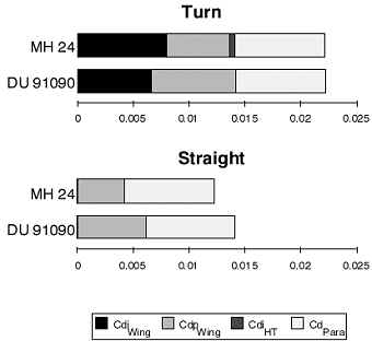
Breakdown of the drag components for the two most important flight conditions (for optimum turns). |
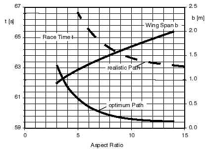
| Changing the aspect ratio of a wing while keeping the wing area constant means an increase in wing span. While this is convenient to reduce the induced drag, the wing chord decreases also. Thus the Reynolds number gets smaller and the friction drag increases. Therefore we can expect, that there is an optimum aspect ratio for a given airfoil. the graph on the right shows the variation of the race time versus aspect ratio and also the corresponding wing spans. For each aspect ratio, the optimum lift coefficient for the turns was used. It seems to be possible to get better results by using extremely long wings, but at aspect ratios above 10, the possible improvements are only very small. Considering a solid wing structure, aspect ratios between 7 and 9 seem to be a good compromise. |
|
| Of course, the power supplied by engine and propeller in terms of thrust is one of the most important parameters. Assuming a pessimistic value of 55% for the combined propeller and installation efficiency, the next figure was created. For each power setting, the optimum lift coefficient for the turns was used. We can see, that the gain due to power is getting quite small at power settings above 3 kW, but there is still an improvement possible. Also the high speeds, which are possible with power of more than 3 kW, force the pilot to make tight turns, so that the airframe reaches its limits in terms of Cl max. While modern engines have not yet reached this limit, it might happen in the future and flaps might become necessary to use the power efficiently on the course. |
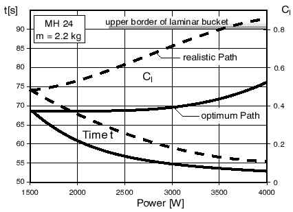
Influence of engine power of race times and optimum lift coefficient. |
Increasing the power from 2 to 2.2 kW reduces the race time by 1.6 seconds, but an increase from 2.8 to 3 kW shortens the time by half that amount only.
The following table, listing three typical conditions, shows that higher temperatures and altitudes give higher race times. This worsening is mainly a result of the power decrease of the engine, and it can be assumed, that a temperature rise by 15 K costs about 1 second in time. The same is true for an increase of the altitude by 500 meters.
| Standard Conditions | High | High & Hot | |
|---|---|---|---|
| Altitude above SL | 0 m | 500 m | 500 m |
| Temperature | 288.15 K | 288.15 K | 303.15 K |
| Density of Air | 1.225 kg/m³ | 1.154 kg/m³ | 1.097 kg/m³ |
| Engine Power | 100% | 94% | 90% |
| Optimum Lift Coefficient | 0.377 | 0.402 | 0.423 |
| Race Time | 60.5 s | 61.3 s | 62.1 s |
As shown in [flaps for pylon racing models], flaps can improve the lap times of a pylon racing model, if the drag polar of the airfoil has a narrow low drag laminar bucket. A comparison with flight test data, recorded by Robbert van den Bosch in the Netherlands, shows, that the simulation is not very far from reality. The only change in the simulation was an adjustment of the rolling resistance for the aircraft on the ground, as the simulated model was accelerating faster than the real model. Static thrust was assumed to be 30 N and the zero thrust speed set to 100 m/s.
The curve for the airfoil with flaps and a lift coefficient of CL=0.55 in the turns (dark blue) matches the experiments very well. The lift coefficient of CL=0.55 was chosen according to the recorded vertical acceleration in the turns, which was in the order of 33...35g. Further analysis of optimized turns show, that the flapped airfoil can be used to turn even more tight, with lift coefficients of CL=0.726 and above (light blue). The average speed for the optimal turns is lower, than the flight test data, but also the distance flown ist smaller and thus the overall flight times are smaller. For the unflapped airfoil, a lift coefficient of CL=0.633 gives the best result (orange curve), which is about 0.5 s slower than the value for the flapped airfoil.
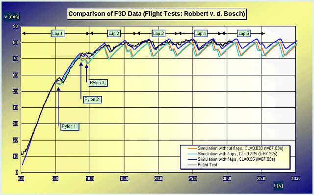
Speed versus time for different configurations of a model
with the DU 91090 airfoil.
Airfoils for Quickie 500 ModelsThe Quickie 500 is not defined as an FAI class contest, but it is widely flown in the USA as well as in Europe. The model is versatile, easy to build and a good introduction into the pylon racing sport. A Q500 model is much simpler and cheaper than an F3D model, but today, the equipment (engine and RC) is not much different from FAI class models. Due to the open engine installation and the omission of a tuned pipe, handling and maintenance of the engine is greatly simplified. Until recently the German rules enforced a prescribed fuselage geometry, similar to the early US rules. Airfoil SelectionFor the Quickie 500 the shape of the model is fairly well prescribed, but the airfoil selection is up to the builder. For the wing, all kinds of airfoils are used. In Germany the Eppler E 220 and the MH 18 airfoils are often used, whereas in the USA the R 140 is often used. Unfortunately I was unable to find the original source for the R 140 coordinates, and had to copy some coordinates from the internet [see the UIUC web site]. These coordinates were quite wavy and had to be smoothed slightly to get useable numerical results. The R 140 is nearly symmetrical and his polars extend far into the negative Cl range. This is not necessary for a pylon racing model and limits the extent of the low drag region at positive lift coefficients. Due to the large, prescribed airfoil thickness of the Q500, this effect is not so important, though. More recent publications, dealing with Q500 airfoils are not known to the author, but in [30] the S 8052 was presented as an improvement of the R 140. Additionally a derivative of the MH 18, with improved low Cl performance, the MH 18B, is available. |
 A selection of possible candidates for a Quickie 500 wing. |
| The graph on the right shows race times for a Quickie 500
and variety of airfoils. These times were calculated with the simulation
program, as described above. Again, airfoil data were calculated with XFOIL
5.4, covering the Reynolds number range from 200'000 to 1'400'000. For each
airfoil, the optimum turn radius was used. First the lines show clearly, how
the mass of the model is directly responsible for the race time: the tribute
to 200 grams of additional mass is one second in race time - the lighter a
model, the better.
Additionally, two groups of airfoils can be identified: the sections E
168, E 220, S 8052 und MH 18 lead to race times which are 1 to 1.5 seconds
higher that the times resulting from the R 140, MH 27 und MH 18B. All the
airfoils in the first group seem to have a problem either with the low Cl
high speed flight (dropping out of the lower border of the laminar bucket)
or with the turns (dropping out of the upper border of the laminar bucket). |
 Race times for different Q500 airfoils versus the mass of the model. |
Often the question is asked, whether the surface quality of the wing does really matter for a Quickie 500 model. Some models are covered with paper and not very carefully sanded, others sport a wrinkled plastic film finish and finally some come with a shiny all composite finish. To get some feeling for the effect, race times for a Quickie 500 with an R 140 airfoil were calculated. The first calculation was done for a smooth surface, with natural transition. A second calculation was performed, assuming transition at 10% of the wing chord (for example forced by a thick, painted trim strip). In real life, the results will probably fall somewhere in between these two extremes. The results show, that a smooth surface, also without much waviness, is awarded with up to 5 seconds in race time. This should be well worth the additional work for a good surface finish!
| Configuration | Lift Coefficient during the Turns | Race Time |
|---|---|---|
| Quickie 500, R140, free transition | 0.275 | 67.3 seconds |
| Quickie 500, R140, transition at 10% x/c | 0.273 | 72.5 seconds |
Last modification of this page: 21.05.18
![]()
[Back to Home Page] Suggestions? Corrections? Remarks? e-mail: Martin Hepperle.
Due to the increasing amount of SPAM mail, I have to change this e-Mail address regularly. You will always find the latest version in the footer of all my pages.
It might take some time until you receive an answer
and in some cases you may even receive no answer at all. I apologize for this, but
my spare time is limited. If you have not lost patience, you might want to send
me a copy of your e-mail after a month or so.
This is a privately owned, non-profit page of purely educational purpose.
Any statements may be incorrect and unsuitable for practical usage. I cannot take
any responsibility for actions you perform based on data, assumptions, calculations
etc. taken from this web page.
© 1996-2018 Martin Hepperle
You may use the data given in this document for your personal use. If you use this
document for a publication, you have to cite the source. A publication of a recompilation
of the given material is not allowed, if the resulting product is sold for more
than the production costs.
This document may accidentally refer to trade names and trademarks, which are owned by national or international companies, but which are unknown by me. Their rights are fully recognized and these companies are kindly asked to inform me if they do not wish their names to be used at all or to be used in a different way.
This document is part of a frame set and can be found by navigating from the entry point at the Web site http://www.MH-AeroTools.de/.